C++ Wavelet Libraries

Documentation

Download

1 Overview

• 1D DWT and IDWT Implementation (Two Modes)
• 2D DWT and IDWT Implementation (Two Modes)
• 1D SWT and ISWT Implementation ( Stationary Wavelet Transform)
• 2D SWT Implementation
• Implemented using FFTW3 Library
• Shared(.so) and static(.a) libraries for Linux
• Shared(.dll) and static(.a) libraries for Win32 GCC (MinGW).
• Shared(.dll) libraries for Microsoft VC++

1.1 Changes from previous version

• FFTW3 Library is used to improve computation speed.
• No GNUPLOT outputs are generated.
• Periodic and Symmetric functions take same arguments. They will still be accessed by the same names, though.(dwt ,dwt_sym etc.)
• Focus on shared libraries. No static libraries for MSVC++ although MinGW and LINUX version will come with static as well as shared libraries.

1.2 Wavelet Libraries in Win32 Environment

1.2.1 Microsoft Visual C++

• Header File- wavelet2d.h
• Import Library- wavelet2d.lib
• Wavelet DLL - wavelet2d.dll
• FFTW DLL - libfftw3-3.dll

1.2.2 GNU-GCC (MinGW) Based Compilation

• Header Files- wavelet2d.h
• Import Library- libwavelet2d.dll.a
• Wavelet DLL - libwavelet2d.dll
• FFTW DLL - libfftw3-3.dll (Import library is also included)

1.3 Working in LINUX Environment

1. This package contains two wavelet libraries- libwavelet2d.so.1.0 (shared) and libwavelet2s.a (static) compiled essentially from the same source code. Source code is available in the ’src’ folder.
2. You may need to link to header files that are included with their resepctive libraries. They are also available in the ’src’ folder.
3. You may want to install shared library in one of your existing paths to make compilation easier. You can create sym links once inside the folder( say /usr/local/lib) by using following commands

• ln -sf libwavelet2d.so.1.0 libwavelet2d.so
• ln -sf libwavelet2d.so.1.0 libwavelet2d.so.1
• ldconfig

You will probably need superuser privileges to perform previous steps. If you don't have su privilege then you can move libwavelet2d.so.1.0 to your work folder or where your source code is, create sym links as before and then put your folder in the path during runtime.

• ln -sf libwavelet2d.so.1.0 libwavelet2d.so
• ln -sf libwavelet2d.so.1.0 libwavelet2d.so.1
• export LD_LIBRARY_PATH=.

libwavelet2s.a Working with static library is pretty straightforward. You will only need to include wavelet2s.h in your program and specify the library (-lwavelet2s flag) , include path (-I[path to wavelet2s.h] flag) and library path (-L[path to libwavelet2s.a] flag).

1.4 Licensing

/*Copyright (C) 2011 Rafat Hussain

This program is free software; you can redistribute it and/or modify it under the terms of the GNU General Public License as published by the Free Software Foundation; version 2 or any later version.This program is distributed in the hope that it will be useful, but WITHOUT ANY WARRANTY; without even the implied warranty of MERCHANTABILITY or FITNESS FOR A PARTICULAR PURPOSE. See the GNU General Public License for more details. You should have received a copy of the GNU General Public License along with this program; if not, write to the Free Software Foundation, Inc., 51 Franklin Street, Fifth Floor, Boston, MA 02110-1301, USA.

2 List of Functions

2.1 1D DWT/IDWT Functions

Periodic Extension

• flag[0] is 0 if the signal is even and it is 1 if signal is odd and if it is made even by repeating the last value one more time
• flag[1] - contains the decomposition levels.

Figure 2.1 DWT stats (periodic extension) for an input signal of length 256

Symmetric Extension

• flag[0] is 0 if the signal is even and it is 1 if signal is odd and if it is made even by repeating the last value one more time
• flag[1] - contains the decomposition levels.

Figure 2.2 DWT stats (symmetric extension) for an input signal of length 256

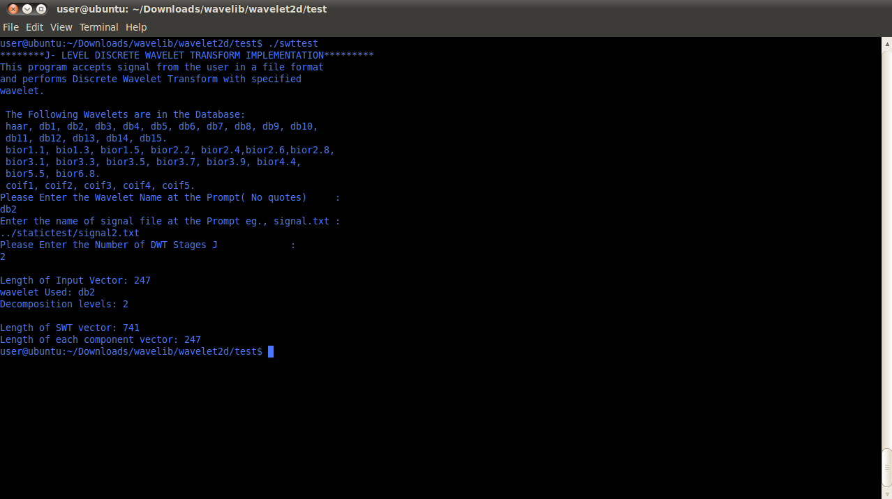
2.2 1D SWT/ISWT Functions

Figure 2.3 Two Level SWT Decomposition of a 247 length signal vector

2.3 2D DWT/IDWT Functions

Periodic Extension

Figure 2.4 2D DWT computation using periodic extension

Symmetric Extension

Figure 2.5 2D DWT computation using symmetric extension

2.4 2D SWT Functions

2.5 Convolution

2.6 Wavelet Filters

2.7 1D Vector Manipulation

2.8 2D Vector Manipulation

3 Sample Codes

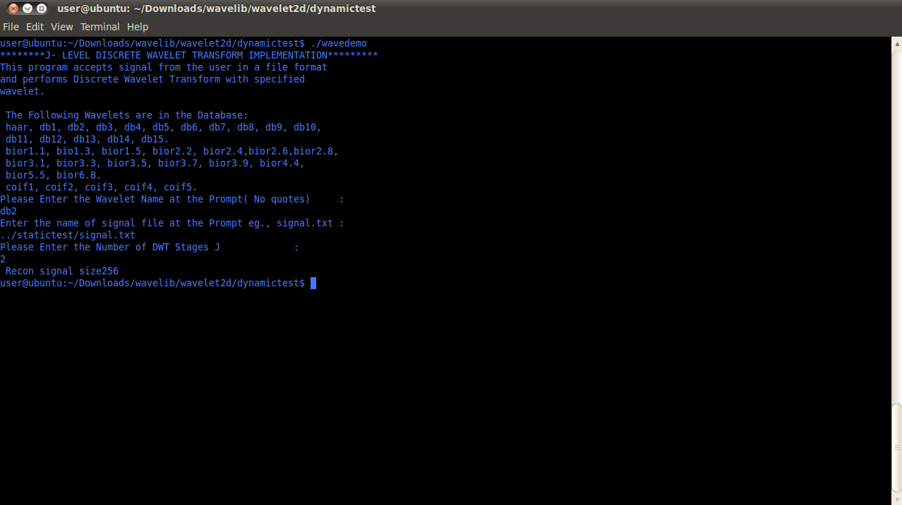
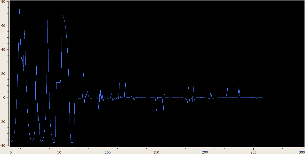
3.1 1D DWT/IDWT Example Code

//=================================================================

// Name : wavedemo1.cpp

// Author :

// Version :

// Copyright :

// Description : 1D DWT Demo

//==============================================================

#include <iostream>

#include <fstream>

#include "wavelet2d.h"

#include <vector>

#include <string>

#include <cmath>

using namespace std;

int main() {

cout << "********J- LEVEL DISCRETE WAVELET TRANSFORM IMPLEMENTATION*********" << endl;

cout << "This program accepts signal from the user in a file format " << endl;

cout << "and performs Discrete Wavelet Transform with specified " << endl;

cout << "wavelet. " << endl;

cout << " " << endl;

cout << " The Following Wavelets are in the Database: " << endl;

cout << " haar, db1, db2, db3, db4, db5, db6, db7, db8, db9, db10, " << endl;

cout << " db11, db12, db13, db14, db15. " << endl;

cout << " bior1.1, bio1.3, bior1.5, bior2.2, bior2.4,bior2.6,bior2.8, " << endl;

cout << " bior3.1, bior3.3, bior3.5, bior3.7, bior3.9, bior4.4," << endl;

cout << " bior5.5, bior6.8." << endl;

cout << " coif1, coif2, coif3, coif4, coif5." << endl;

cout << "Please Enter the Wavelet Name at the Prompt( No quotes) :" << endl;

string nm; // nm will store the name of Wavelet Family

cin >> nm;

cout << "Enter the name of signal file at the Prompt eg., signal.txt :" << endl;

char inp[50];

cin >> inp;

vector<double> sig;

ifstream sig_inp(inp);

if ( !sig_inp.good()){

cout << "The File doesn’t exist"<< endl;

}

while (sig_inp) {

double temp;

sig_inp >> temp;

sig.push_back(temp);

}

sig.pop_back();

vector<double> original;

original = sig;

cout << "Please Enter the Number of DWT Stages J :" << endl;

int J;

cin >> J ;

vector<double> dwt_output, flag;

// perform J-Level DWT

vector<int> length;

dwt_sym(sig, J, nm, dwt_output,flag,length);

ofstream dwtout("dwtout.txt");

for (unsigned int i = 0; i < dwt_output.size(); i++){

dwtout << dwt_output[i] << endl;

}

//Perform J-Level IDWT

vector<double> output;

idwt_sym(dwt_output, flag,nm,output,length);

ofstream sig1("recon.txt");

ofstream diff("diff.txt");

cout <<" Recon signal size" << output.size() << endl;

for (unsigned int i = 0; i < output.size(); i++){

sig1 << output[i] << endl;

diff << output[i] - original[i] << endl;

}

//gnudwtplot(J);

return 0;

}

Figure 3.1 1D DWT Console

Figure 3.2 Length 256 Piecewise Regular signal from WaveLab

Figure 3.3 2 Level DWT Decomposition Coefficients obtained using db2 wavelet

Figure 3.4 Reconstructed Signal After IDWT computations

3.2 1D Linear vs Nonlinear Approximation

//===============================================================

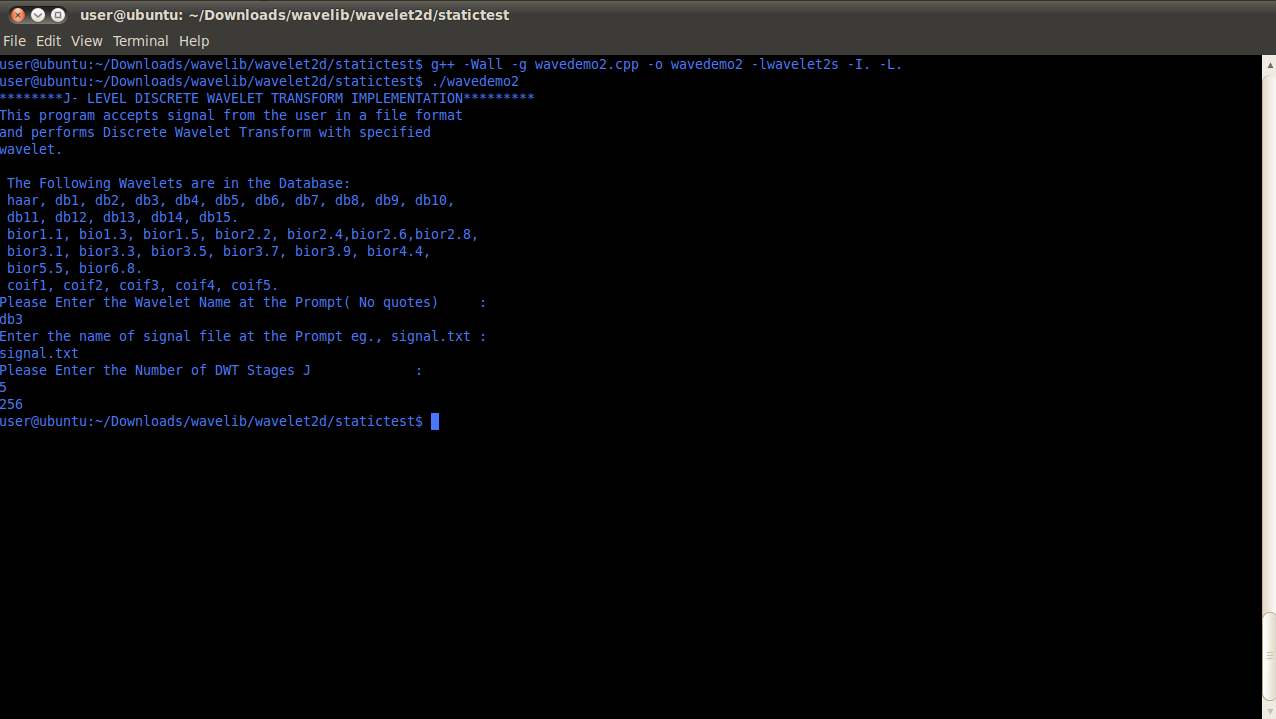
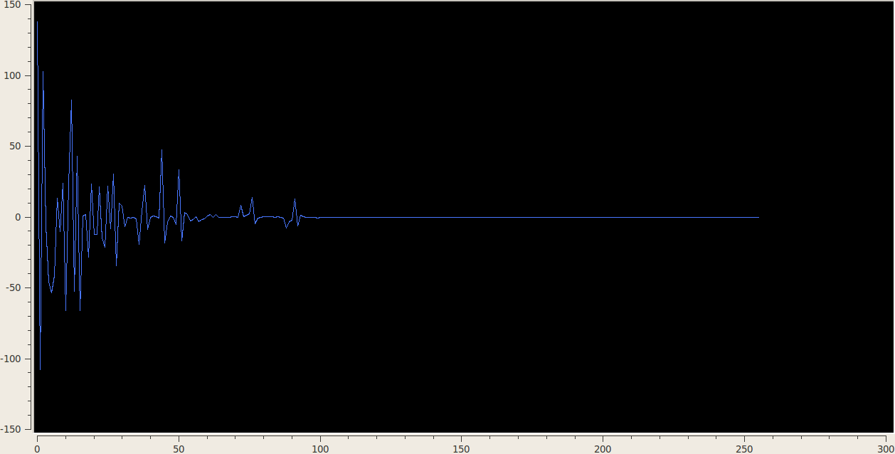
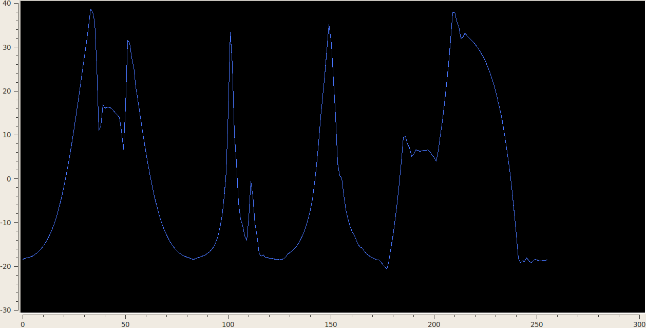
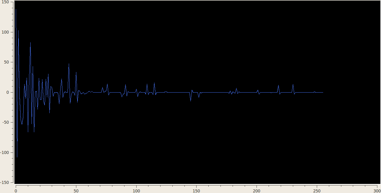
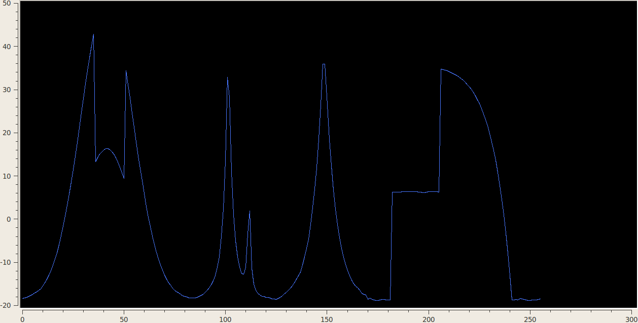
// Name : wavedemo2.cpp

// Author :

// Version :

// Copyright :

// Description : Wavelet Demo comparing linear and non-linear approximation properties

// : of a given wavelet. Implemented using dwt_sym and idwt_sym.

//============================================================

#include <iostream>

#include <fstream>

#include "wavelet2s.h"

#include <vector>

#include <string>

#include <cmath>

#include <algorithm>

using namespace std;

void findthresh(vector<double> vector1, int N, double& t){

sort(vector1.begin(), vector1.end(), greater<double>());

t = vector1.at(N-1);

}

int main() {

cout << "********J- LEVEL DISCRETE WAVELET TRANSFORM IMPLEMENTATION*********" << endl;

cout << "This program accepts signal from the user in a file format " << endl;

cout << "and performs Discrete Wavelet Transform with specified " << endl;

cout << "wavelet. " << endl;

cout << " " << endl;

cout << " The Following Wavelets are in the Database: " << endl;

cout << " haar, db1, db2, db3, db4, db5, db6, db7, db8, db9, db10, " << endl;

cout << " db11, db12, db13, db14, db15. " << endl;

cout << " bior1.1, bio1.3, bior1.5, bior2.2, bior2.4,bior2.6,bior2.8, " << endl;

cout << " bior3.1, bior3.3, bior3.5, bior3.7, bior3.9, bior4.4," << endl;

cout << " bior5.5, bior6.8." << endl;

cout << " coif1, coif2, coif3, coif4, coif5." << endl;

cout << "Please Enter the Wavelet Name at the Prompt( No quotes) :" << endl;

string nm; // nm will store the name of Wavelet Family

cin >> nm;

cout << "Enter the name of signal file at the Prompt eg., signal.txt :" << endl;

char inp[50];

cin >> inp;

vector<double> sig;

ifstream sig_inp(inp);

if ( !sig_inp.good()){

cout << "The File doesn’t exist"<< endl;

exit(1);

}

while (sig_inp) {

double temp;

sig_inp >> temp;

sig.push_back(temp);

}

sig.pop_back();

vector<double> original;

original = sig;

cout << "Please Enter the Number of DWT Stages J :" << endl;

int J;

cin >> J ;

vector<double> dwt_output, flag;

vector<int> length1;

// perform J-Level DWT

dwt(sig, J, nm, dwt_output,flag, length1);

// Performing Linear Approximation by using only first 100 coefficients

// Coefficients in dwt_output are stored as following

// dwt_output =[ Appx(J-1) Detail(J-1) Detail(J-2) .... Detail(0)]

int n_coef = 100; // Number of significant coefficients

int n_non_sig= dwt_output.size() - n_coef; // Number of Coefficients that will

// be set to zero

dwt_output.erase(dwt_output.end()- n_non_sig,dwt_output.end());

// Deleting last n_non_sig coefficients and replacing them with zeros

dwt_output.insert(dwt_output.end(),n_non_sig,0);

ofstream linearsig("linsig.txt");

for (unsigned int i = 0; i < dwt_output.size(); i++) {

linearsig << dwt_output[i] << endl;

}

// Finding IDWT with approximated coefficients

vector<double> output;

idwt(dwt_output, flag,nm,output, length1);

unsigned int count = output.size();

ofstream gnulinappx("gnulinappx.dat");

for (unsigned int i = 0;i < count; i++) {

gnulinappx << output[i] << endl;

}

gnulinappx.close();

// Performing Non Linear Approximation by using only most

// significant coefficients

vector<double> dwt_output2, flag2;

vector<int> length2;

// perform J-Level DWT

dwt(sig, J, nm, dwt_output2,flag2,length2);

double thresh = 0.0;

vector<double> temp_dwtoutput;

for (unsigned int i =0; i < dwt_output2.size();i++){

double temp = abs(dwt_output2[i]);

temp_dwtoutput.push_back(temp);

}

/*

for (unsigned int i =0; i < temp_dwtoutput.size(); i++){

cout << temp_dwtoutput[i] << endl;

}

*/

findthresh(temp_dwtoutput,n_coef, thresh);

for (unsigned int i = 0; i < dwt_output2.size();i++){

double temp = abs(dwt_output2[i]);

if (temp < thresh){

dwt_output2.at(i) = 0.0;

}

}

/*

for (unsigned int i =0; i < dwt_output2.size(); i++){

cout << dwt_output2[i] << endl;

}

*/

ofstream nonlinsig("nonlinsig.txt");

for (unsigned int i = 0; i < dwt_output2.size(); i++) {

nonlinsig << dwt_output2[i] << endl;

}

// Finding IDWT with approximated coefficients

vector<double> output2;

idwt(dwt_output2, flag2,nm,output2, length2);

unsigned int count2 = output2.size();

cout << count2 << endl;

ofstream gnunlappx("gnunlappx.dat");

for (unsigned int i = 0;i < count2; i++) {

gnunlappx << output2[i] << endl;

}

gnunlappx.close();

return 0;

}

Figure 3.5 Console showing db3 5 level computation

Figure 3.6 Length 256 Piecewise Regular signal from WaveLab

Figure 3.7 Retained Coefficients for Linear Approximation case

Figure 3.8 Reconstructed Signal using Linear Approximation

Figure 3.9 Retained Coefficients(Non-Linear Approximation case)

Figure 3.10 Reconstructed Signal(Non-Linear Approximation Case)

3.3 1D Stationary Wavelet Transform

//===========================================================

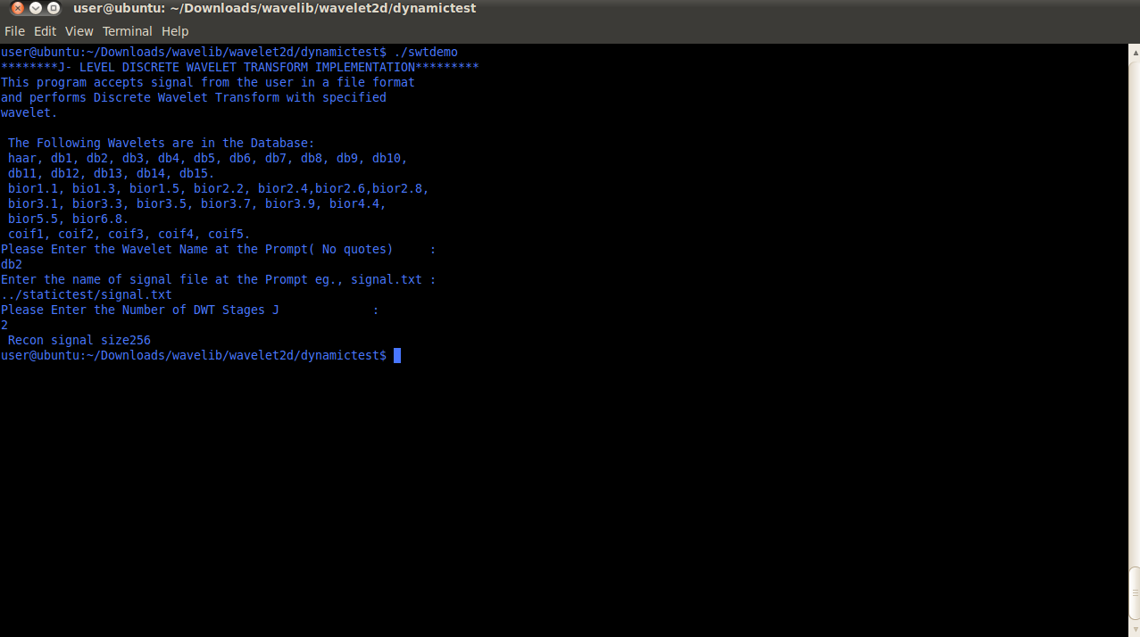
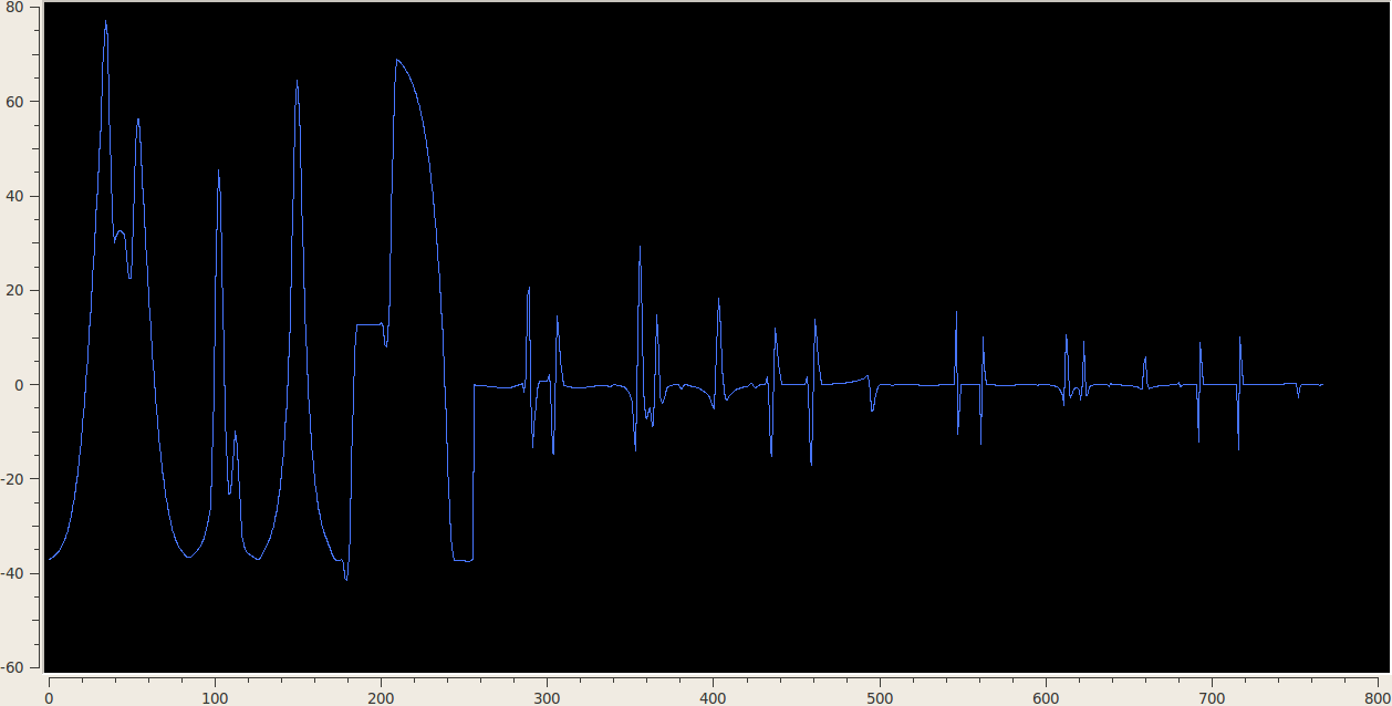
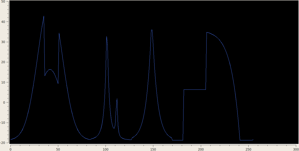
// Name : swtdemo.cpp

// Author :

// Version :

// Copyright :

// Description : 1D Stationary Wavelet Transform Demo

//=========================================================

#include <iostream>

#include <fstream>

#include "wavelet2d.h"

#include <vector>

#include <string>

#include <cmath>

using namespace std;

int main() {

cout << "********J- LEVEL DISCRETE WAVELET TRANSFORM IMPLEMENTATION*********" << endl;

cout << "This program accepts signal from the user in a file format " << endl;

cout << "and performs Discrete Wavelet Transform with specified " << endl;

cout << "wavelet. " << endl;

cout << " " << endl;

cout << " The Following Wavelets are in the Database: " << endl;

cout << " haar, db1, db2, db3, db4, db5, db6, db7, db8, db9, db10, " << endl;

cout << " db11, db12, db13, db14, db15. " << endl;

cout << " bior1.1, bio1.3, bior1.5, bior2.2, bior2.4,bior2.6,bior2.8, " << endl;

cout << " bior3.1, bior3.3, bior3.5, bior3.7, bior3.9, bior4.4," << endl;

cout << " bior5.5, bior6.8." << endl;

cout << " coif1, coif2, coif3, coif4, coif5." << endl;

cout << "Please Enter the Wavelet Name at the Prompt( No quotes) :" << endl;

string nm; // nm will store the name of Wavelet Family

cin >> nm;

cout << "Enter the name of signal file at the Prompt eg., signal.txt :" << endl;

char inp[50];

cin >> inp;

vector<double> sig;

ifstream sig_inp(inp);

if ( !sig_inp.good()){

cout << "The File doesn’t exist"<< endl;

}

while (sig_inp) {

double temp;

sig_inp >> temp;

sig.push_back(temp);

}

sig.pop_back();

vector<double> original;

original = sig; // Make a copy of the signal if you want to use original signal

// later on. The other option is to use IDWT output as the SWt/ISWT system is

// Perefect Reconstruction system.

cout << "Please Enter the Number of DWT Stages J :" << endl;

int J;

cin >> J ;

vector<double> swt_output;

// perform J-Level DWT

int length;// All coefficients are of same length. Variable "length" returns length

// of coefficients. It is not required for ISWT computations.

// If signal is not of dyadic length it is zeropadded as the algorithm is designed to

// work with signals of 2^M length. These extra zeros can be removed after reconstruction

swt(sig, J, nm, swt_output, length);

ofstream swtcoeff("swtcoeff.txt");

for (unsigned int i=0; i < swt_output.size(); i++) {

swtcoeff << swt_output[i] << endl;

}

vector<double> iswt_output;

iswt(swt_output,J, nm,iswt_output);

ofstream sig1("recon.txt");

ofstream diff("diff.txt");

cout <<" Recon signal size" << iswt_output.size() << endl;

for (unsigned int i = 0; i < iswt_output.size(); i++){

sig1 << iswt_output[i] << endl;

diff << iswt_output[i] - original[i] << endl;

}

return 0;

}

Figure 3.11 Console Running swt demo

Figure 3.12 Input Signal(Length-256)

Figure 3.13 SWT Coefficients for two level of Decomposition(Length 3 X 256)

Figure 3.14 SWT Reconstructed Signal

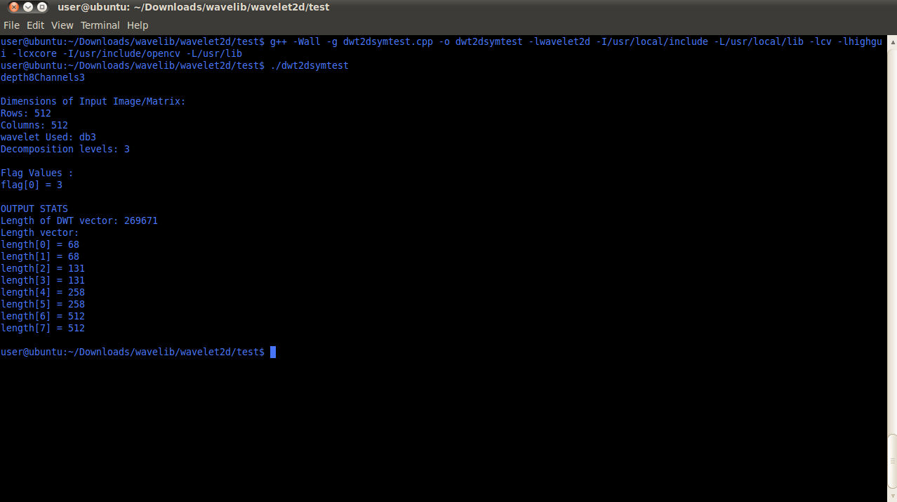
3.4 2D DWT/IDWT Demo Code

//============================================================

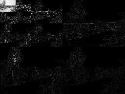
// Name : imagedemo1.cpp

// Author :

// Version :

// Copyright :

// Description : DWT of arbitrary size image using symmetric or periodic extension

//===========================================================

#include <iostream>

#include <fstream>

#include <vector>

#include <string>

#include <complex>

#include <cmath>

#include <algorithm>

#include "wavelet2d.h"

#include "cv.h"

#include "highgui.h"

#include "cxcore.h"

using namespace std;

using namespace cv;

void* maxval(vector<vector<double> > &arr, double &max){

max = 0;

for (unsigned int i =0; i < arr.size(); i++) {

for (unsigned int j =0; j < arr[0].size(); j++) {

if (max <= arr[i][j]){

max = arr[i][j];

}

}

}

return 0;

}

void* maxval1(vector<double> &arr, double &max){

max = 0;

for (unsigned int i =0; i < arr.size(); i++) {

if (max <= arr[i]){

max = arr[i];

}

}

return 0;

}

int main() {

IplImage* img = cvLoadImage("snow.jpg");

if (!img){

cout << " Can’t read Image. Try Different Format." << endl;

exit(1);

}

int height, width;

height = img->height;

width = img->width;

int nc = img->nChannels;

// uchar* ptr2 =(uchar*) img->imageData;

int pix_depth = img->depth;

CvSize size;

size.width =width;

size.height=height;

cout << "depth" << pix_depth << "Channels" << nc << endl;

cvNamedWindow("Original Image", CV_WINDOW_AUTOSIZE);

cvShowImage("Original Image", img);

cvWaitKey();

cvDestroyWindow("Original Image");

cvSaveImage("orig.bmp",img);

int rows =(int) height;

int cols =(int) width;

Mat matimg(img);

vector<vector<double> > vec1(rows, vector<double>(cols));

int k =1;

for (int i=0; i < rows; i++) {

for (int j =0; j < cols; j++){

unsigned char temp;

temp = ((uchar*) matimg.data + i * matimg.step)[j * matimg.elemSize() + k ];

vec1[i][j] = (double) temp;

}

}

string nm = "db3";

vector<double> l1,h1,l2,h2;

filtcoef(nm,l1,h1,l2,h2);

// unsigned int lf=l1.size();

// int rows_n =(int) (rows+ J*(lf-1));

// int cols_n =(int) (cols + J * ( lf -1));

// Finding 2D DWT Transform of the image using symetric extension algorithm

// Extension is set to 3 (eg., int e = 3)

vector<int> length;

vector<double> output,flag;

int J =3;

dwt_2d_sym(vec1,J,nm,output,flag,length);

double max;

vector<int> length2;

// This algorithm computes DWT of image of any given size. Together with convolution and

// subsampling operations it is clear that subsampled images are of different length than

// dyadic length images. In order to compute the "effective" size of DWT we do additional

// calculations.

dwt_output_dim_sym(length,length2,J);

// length2 is gives the integer vector that contains the size of subimages that will

// combine to form the displayed output image. The last two entries of length2 gives the

// size of DWT ( rows_n by cols_n)

int siz = length2.size();

int rows_n=length2[siz-2];

int cols_n = length2[siz-1];

vector<vector< double> > dwtdisp(rows_n, vector<double>(cols_n));

dispDWT(output,dwtdisp, length ,length2, J);

// dispDWT returns the 2D object dwtdisp which will be displayed using OPENCV’s image

// handling functions

vector<vector<double> > dwt_output= dwtdisp;

maxval(dwt_output,max);// max value is needed to take care of overflow which happens because

// of convolution operations performed on unsigned 8 bit images

//Displaying Scaled Image

// Creating Image in OPENCV

IplImage *cvImg; // image used for output

CvSize imgSize; // size of output image

imgSize.width = cols_n;

imgSize.height = rows_n;

cvImg = cvCreateImage( imgSize, 8, 1 );

// dwt_hold is created to hold the dwt output as further operations need to be

// carried out on dwt_output in order to display scaled images.

vector<vector<double> > dwt_hold(rows_n, vector<double>( cols_n));

dwt_hold = dwt_output;

// Setting coefficients of created image to the scaled DWT output values

for (int i = 0; i < imgSize.height; i++ ) {

for (int j = 0; j < imgSize.width; j++ ){

if ( dwt_output[i][j] <= 0.0){

dwt_output[i][j] = 0.0;

}

if ( i <= (length2[0]) && j <= (length2[1]) ) {

((uchar*)(cvImg->imageData + cvImg->widthStep*i))[j] =

(char) ( (dwt_output[i][j] / max) * 255.0);

} else {

((uchar*)(cvImg->imageData + cvImg->widthStep*i))[j] =

(char) (dwt_output[i][j]) ;

}

}

}

cvNamedWindow( "DWT Image", 1 ); // creation of a visualisation window

cvShowImage( "DWT Image", cvImg ); // image visualisation

cvWaitKey();

cvDestroyWindow("DWT Image");

cvSaveImage("dwt.bmp",cvImg);

// Finding IDWT

vector<vector<double> > idwt_output(rows, vector<double>(cols));

idwt_2d_sym(output,flag, nm, idwt_output,length);

//Displaying Reconstructed Image

IplImage *dvImg;

CvSize dvSize; // size of output image

dvSize.width = idwt_output[0].size();

dvSize.height = idwt_output.size();

cout << idwt_output.size() << idwt_output[0].size() << endl;

dvImg = cvCreateImage( dvSize, 8, 1 );

for (int i = 0; i < dvSize.height; i++ )

for (int j = 0; j < dvSize.width; j++ )

((uchar*)(dvImg->imageData + dvImg->widthStep*i))[j] =

(char) (idwt_output[i][j]) ;

cvNamedWindow( "Reconstructed Image", 1 ); // creation of a visualisation window

cvShowImage( "Reconstructed Image", dvImg ); // image visualisation

cvWaitKey();

cvDestroyWindow("Reconstructed Image");

cvSaveImage("recon.bmp",dvImg);

return 0;

}

Figure 3.15 Input 250X189 Image

Figure 3.16 3-Level Decomposition using db3 wavelet

Figure 3.17 Reconstructed Image

3.5 Image Approximation Demo

//============================================================

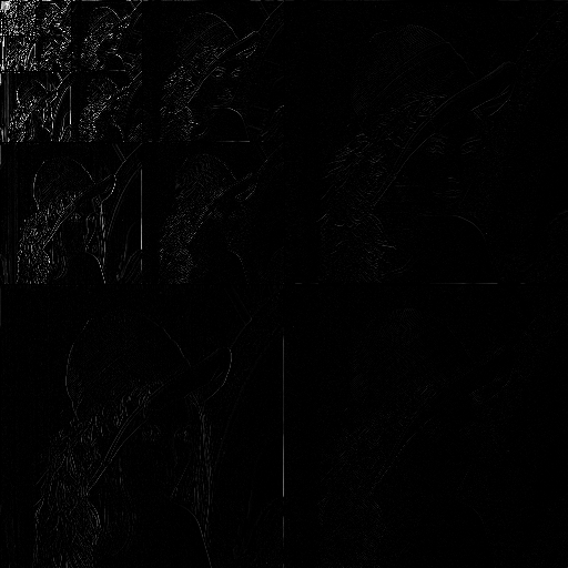
// Name : imagedemo2.cpp

// Author :

// Version :

// Copyright :

// Description : Image Approximation using symmetric extension 2D DWT

//=========================================================

// IMPORTANT - Algorithm used to display Image is imprecise because of int 8 overflow issues

// and it shouldn’t be used to judge the performance of the DWT. The DWT and IDWT outputs

// should be used for performance measurements. I have used maximum value rescaling to

// solve overflow issues and , obviously, it is going to result in suboptimal performance but

// it is good enough for demonstration purposes.

#include <iostream>

#include <fstream>

#include <vector>

#include <string>

#include <complex>

#include <cmath>

#include <algorithm>

#include "wavelet2s.h"

#include "cv.h"

#include "highgui.h"

#include "cxcore.h"

using namespace std;

using namespace cv;

void findthresh(vector<double> &vector1, int N, double& t){

sort(vector1.begin(), vector1.end(), greater<double>());

t = vector1.at(N-1);

}

void* maxval(vector<vector<double> > &arr, double &max){

max = 0;

for (unsigned int i =0; i < arr.size(); i++) {

for (unsigned int j =0; j < arr[0].size(); j++) {

if (max <= arr[i][j]){

max = arr[i][j];

}

}

}

return 0;

}

void* maxval1(vector<double> &arr, double &max){

max = 0;

for (unsigned int i =0; i < arr.size(); i++) {

if (max <= arr[i]){

max = arr[i];

}

}

return 0;

}

int main() {

IplImage* img = cvLoadImage("lena512.bmp");

if (!img){

cout << " Can’t read Image. Try Different Format." << endl;

exit(1);

}

int height, width;

height = img->height;

width = img->width;

int nc = img->nChannels;

// uchar* ptr2 =(uchar*) img->imageData;

int pix_depth = img->depth;

CvSize size;

size.width =width;

size.height=height;

cout << "depth" << pix_depth << "Channels" << nc << endl;

cvNamedWindow("Original Image", CV_WINDOW_AUTOSIZE);

cvShowImage("Original Image", img);

cvWaitKey();

cvDestroyWindow("Original Image");

cvSaveImage("orig.bmp",img);

int rows =(int) height;

int cols =(int) width;

Mat matimg(img);

vector<vector<double> > vec1(rows, vector<double>(cols));

int k =1;

for (int i=0; i < rows; i++) {

for (int j =0; j < cols; j++){

unsigned char temp;

temp = ((uchar*) matimg.data + i * matimg.step)[j * matimg.elemSize() + k ];

vec1[i][j] = (double) temp;

}

}

string nm = "db2";

vector<double> l1,h1,l2,h2;

filtcoef(nm,l1,h1,l2,h2);

// unsigned int lf=l1.size();

// int rows_n =(int) (rows+ J*(lf-1));

// int cols_n =(int) (cols + J * ( lf -1));

// Finding 2D DWT Transform of the image using symetric extension algorithm

// Extension is set to 0 (eg., int e = 0)

vector<int> length;

vector<double> output,flag;

int J =6;

dwt_2d(vec1,J,nm,output,flag,length);

double max;

vector<int> length2;

// This algorithm computes DWT of image of any given size. Together with convolution and

// subsampling operations it is clear that subsampled images are of different length than

// dyadic length images. In order to compute the "effective" size of DWT we do additional

// calculations.

dwt_output_dim_sym(length,length2,J);

// length2 is gives the integer vector that contains the size of subimages that will

// combine to form the displayed output image. The last two entries of length2 gives the

// size of DWT ( rows_n by cols_n)

int siz = length2.size();

int rows_n=length2[siz-2];

int cols_n = length2[siz-1];

vector<vector< double> > dwtdisp(rows_n, vector<double>(cols_n));

dispDWT(output,dwtdisp, length ,length2, J);

// dispDWT returns the 2D object dwtdisp which will be displayed using OPENCV’s image

// handling functions

vector<vector<double> > dwt_output= dwtdisp;

// Storing the DWT coefficients in two different vectors that will be used to approximate

// Image with two different sets of chosen coefficients.

vector<double> dwt_coef1;

vector<double> dwt_coef2;

dwt_coef1 = output;

dwt_coef2 = output;

maxval(dwt_output,max);// max value is needed to take care of overflow which happens because

// of convolution operations performed on unsigned 8 bit images

//Displaying Scaled Image

// Creating Image in OPENCV

IplImage *cvImg; // image used for output

CvSize imgSize; // size of output image

imgSize.width = cols_n;

imgSize.height = rows_n;

cvImg = cvCreateImage( imgSize, 8, 1 );

// dwt_hold is created to hold the dwt output as further operations need to be

// carried out on dwt_output in order to display scaled images.

vector<vector<double> > dwt_hold(rows_n, vector<double>( cols_n));

dwt_hold = dwt_output;

// Setting coefficients of created image to the scaled DWT output values

for (int i = 0; i < imgSize.height; i++ ) {

for (int j = 0; j < imgSize.width; j++ ){

if ( dwt_output[i][j] <= 0.0){

dwt_output[i][j] = 0.0;

}

if ( i <= (length2[0]) && j <= (length2[1]) ) {

((uchar*)(cvImg->imageData + cvImg->widthStep*i))[j] =

(char) ( (dwt_output[i][j] / max) * 255.0);

} else {

((uchar*)(cvImg->imageData + cvImg->widthStep*i))[j] =

(char) (dwt_output[i][j]) ;

}

}

}

cvNamedWindow( "DWT Image", 1 ); // creation of a visualisation window

cvShowImage( "DWT Image", cvImg ); // image visualisation

cvWaitKey();

cvDestroyWindow("DWT Image");

cvSaveImage("dwt.bmp",cvImg);

// Case 1 : Only 10% of the largest coefficients are considered

// Output is the 1D DWT vector

int n_coef1= int (output.size()/ 10);

cout << n_coef1 << endl;

// Finding Threshold Value corresponding to n_coef1

vector<double> temp1;

cout << "size: " << (int) temp1.size() << "\n";

cout << "capacity: " << (int) temp1.capacity() << "\n";

cout << "max_size: " << (int) temp1.max_size() << "\n";

for (unsigned int i =0; i < dwt_coef1.size(); i++) {

double tempval = abs(dwt_coef1[i]);

temp1.push_back(tempval);

}

double thresh1= 0.0;

findthresh(temp1,n_coef1,thresh1);

cout << "thresh" << thresh1 << endl;

ofstream temp("temp.txt");

for (unsigned int i =0; i < temp1.size(); i++){

temp << temp1[i] << " " ;

}

// Reset coeffficients value depending on threshold value

for (unsigned int i =0; i < dwt_coef1.size(); i++) {

double temp = abs(dwt_coef1[i]);

if (temp < thresh1){

dwt_coef1.at(i)= 0.0;

}

}

// Finding IDWT

vector<vector<double> > idwt_output(rows, vector<double>(cols));

idwt_2d( dwt_coef1,flag, nm, idwt_output,length);

double max1;

maxval(idwt_output,max1);

//Displaying Reconstructed Image

IplImage *dvImg;

CvSize dvSize; // size of output image

dvSize.width = idwt_output[0].size();

dvSize.height = idwt_output.size();

cout << idwt_output.size() << idwt_output[0].size() << endl;

dvImg = cvCreateImage( dvSize, 8, 1 );

for (int i = 0; i < dvSize.height; i++ ){

for (int j = 0; j < dvSize.width; j++ ){

if ( idwt_output[i][j] <= 0.0){

idwt_output[i][j] = 0.0;

}

((uchar*)(dvImg->imageData + dvImg->widthStep*i))[j] =

(char) ((idwt_output[i][j] / max1) * 255 ) ;

}

}

cvNamedWindow( "10% Coeff Reconstructed Image", 1 ); // creation of a visualisation window

cvShowImage( "10% Coeff Reconstructed Image", dvImg ); // image visualisation

cvWaitKey();

cvDestroyWindow("10% Coeff Reconstructed Image");

cvSaveImage("recon.bmp",dvImg);

// Case 2 : Only 2% of the largest coefficients are considered

// Output is the 1D DWT vector

int n_coef2= int (output.size()/ 50);

cout << n_coef2 << endl;

// Finding Threshold Value corresponding to n_coef1

vector<double> temp2;

for (unsigned int i =0; i < dwt_coef2.size(); i++) {

double tempval = abs(dwt_coef2[i]);

temp2.push_back(tempval);

}

double thresh2= 0.0;

findthresh(temp2,n_coef2,thresh2);

cout << "thresh" << thresh2 << endl;

// Reset coeffficients value depending on threshold value

for (unsigned int i =0; i < dwt_coef2.size(); i++) {

double temp = abs(dwt_coef2[i]);

if (temp < thresh2){

dwt_coef2.at(i)= 0.0;

}

}

// Finding IDWT

vector<vector<double> > idwt_output2(rows, vector<double>(cols));

idwt_2d( dwt_coef2,flag, nm, idwt_output2,length);

double max2;

maxval(idwt_output2,max2);

//Displaying Reconstructed Image

IplImage *dvImg2;

CvSize dvSize2; // size of output image

dvSize2.width = idwt_output2[0].size();

dvSize2.height = idwt_output2.size();

cout << idwt_output2.size() << idwt_output2[0].size() << endl;

dvImg2 = cvCreateImage( dvSize2, 8, 1 );

for (int i = 0; i < dvSize2.height; i++ ) {

for (int j = 0; j < dvSize2.width; j++ ) {

if ( idwt_output2[i][j] <= 0.0){

idwt_output2[i][j] = 0.0;

}

((uchar*)(dvImg2->imageData + dvImg2->widthStep*i))[j] =

(char) ((idwt_output2[i][j]/ max2) * 255 ) ;

}

}

cvNamedWindow( "2% Coeff Reconstructed Image", 1 ); // creation of a visualisation window

cvShowImage( "2% Coeff Reconstructed Image", dvImg2 ); // image visualisation

cvWaitKey();

cvDestroyWindow("2% Coeff Reconstructed Image");

cvSaveImage("recon2.bmp",dvImg2);

return 0;

}

Figure 3.18 Input Image

Figure 3.19 DWT of Input Image

Figure 3.20 2D Approximation using only 1/10th Coefficients

Figure 3.21 2D Approximation using only 1/50th Coefficients

3.6 2D SWT Demo

//==============================================================

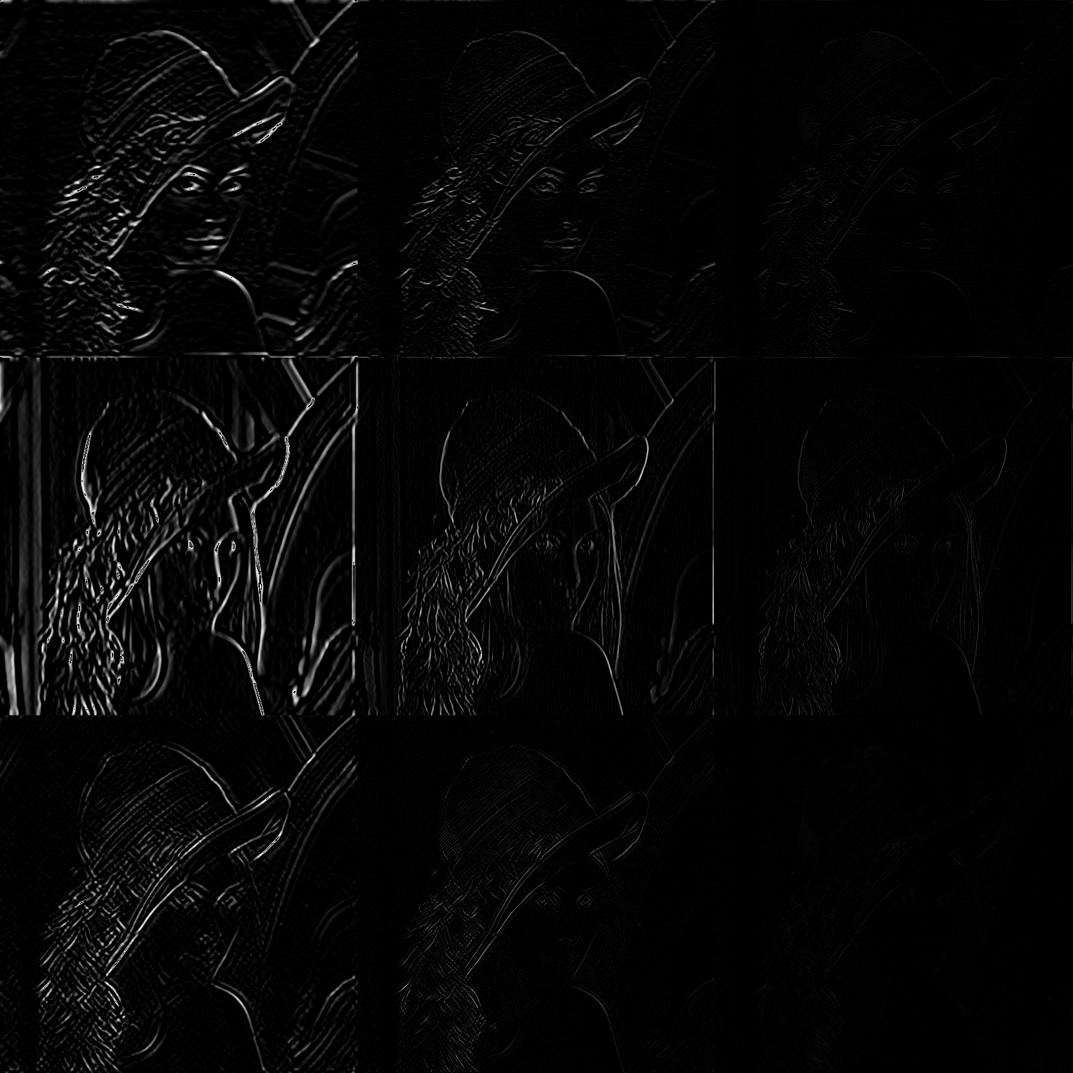
// Name : swt2Ddemo.cpp

// Author :

// Version :

// Copyright :

// Description : 2D SWT Demo using OPENCV

//===========================================================

#include <iostream>

#include <fstream>

#include <vector>

#include <string>

#include <complex>

#include <cmath>

#include <algorithm>

#include "wavelet2d.h"

#include "cv.h"

#include "highgui.h"

#include "cxcore.h"

using namespace std;

using namespace cv;

void* maxval(vector<vector<double> > &arr, double &max){

max = 0;

for (unsigned int i =0; i < arr.size(); i++) {

for (unsigned int j =0; j < arr[0].size(); j++) {

if (max <= arr[i][j]){

max = arr[i][j];

}

}

}

return 0;

}

int main() {

IplImage* img = cvLoadImage("lena512.bmp");

if (!img){

cout << " Can’t read Image. Try Different Format." << endl;

exit(1);

}

int height, width;

height = img->height;

width = img->width;

int nc = img->nChannels;

// uchar* ptr2 =(uchar*) img->imageData;

int pix_depth = img->depth;

CvSize size;

size.width =width;

size.height=height;

cout << "depth" << pix_depth << "Channels" << nc << endl;

cvNamedWindow("Original Image", CV_WINDOW_AUTOSIZE);

cvShowImage("Original Image", img);

cvWaitKey();

cvDestroyWindow("Original Image");

cvSaveImage("orig.bmp",img);

int rows =(int) height;

int cols =(int) width;

Mat matimg(img);

vector<vector<double> > vec1(rows, vector<double>(cols));

int k =1;

for (int i=0; i < rows; i++) {

for (int j =0; j < cols; j++){

unsigned char temp;

temp = ((uchar*) matimg.data + i * matimg.step)[j * matimg.elemSize() + k ];

vec1[i][j] = (double) temp;

}

}

string nm = "db2";

// vector<double> l1,h1,l2,h2;

// filtcoef(nm,l1,h1,l2,h2);

vector<double> output;

int J =3;

swt_2d(vec1,J,nm,output);

cout << "OUTPUT size" << output.size() << endl;

cout << "LOOP OK" << endl;

int row,col;

dwt_output_dim(vec1, row, col );

// Extract and Display Low Pass Image at the Jth stage

vector<vector<double> > blur(row,vector<double>(col));

for (int i=0;i < row; i++){

for (int j=0; j < col;j++){

double temp = output[i*col + j];

blur[i][j]= temp;

}

}

double max;

maxval(blur,max);

// Creating Image in OPENCV

IplImage *cvImg; // image used for output

CvSize imgSize; // size of output image

imgSize.width = col;

imgSize.height = row;

cvImg = cvCreateImage( imgSize, 8, 1 );

for (int i = 0; i < imgSize.height; i++ ) {

for (int j = 0; j < imgSize.width; j++ ){

if ( blur[i][j] <= 0.0){

blur[i][j] = 0.0;

}

((uchar*)(cvImg->imageData + cvImg->widthStep*i))[j] =

(char) ( (blur[i][j] / max) * 255.0);

}

}

cvNamedWindow( "Low Pass Image", 1 ); // creation of a visualisation window

cvShowImage( "Low Pass Image", cvImg ); // image visualisation

cvWaitKey();

cvDestroyWindow("Low Pass Image");

cvSaveImage("blur.bmp",cvImg);

// Displaying BandPass Images

vector<vector<double> > detail(3*row,vector<double>(J * col));

for (int k=0; k < J; k++) {

for (int i=0; i < 3*row; i++) {

for(int j=0+ k*col; j < (k+1)*col; j++) {

double temp = output[(3*k+1)*row*col+ i * col +j - k*col];

detail[i][j]= temp;

}

}

}

IplImage *dvImg; // image used for output

CvSize imgSz; // size of output image

imgSz.width = J*col;

imgSz.height = 3*row;

dvImg = cvCreateImage( imgSz, 8, 1 );

for (int i = 0; i < imgSz.height; i++ ) {

for (int j = 0; j < imgSz.width; j++ ){

if ( detail[i][j] <= 0.0){

detail[i][j] = 0.0;

}

((uchar*)(dvImg->imageData + dvImg->widthStep*i))[j] =

(char) detail[i][j];

}

}

cvNamedWindow( "Band Pass Image", 1 ); // creation of a visualisation window

cvShowImage( "Band Pass Image", dvImg ); // image visualisation

cvWaitKey();

cvDestroyWindow("Band Pass Image");

cvSaveImage("detail.bmp",dvImg);

return 0;

}

Figure 3.22 Input Image

Figure 3.23 Approximation image at Level J = 3

Figure 3.24 Detail Images at levels J=3,2,1(L-R).Horizontal,Vertical,Diagonal(T-B).(Resized)

Copyright (C) Rafat Hussain 2011 Documentation